DTU CO313 CG Midsem

Pixel and Frame Buffer in computer graphics | Lecture 7

Image Processing in computer graphics | picture | Lecture 8

Digital Differential Analyzer(DDA) Line drawing algorithm Part-1 in Hindi with Solved Example

Frame Buffer in Computer Graphics ,frame buffer in computer graphics in Hindi Lecture 10

Frame Buffer : A frame buffers is a large, contiguous piece of memory. Then intensity values for all pixels are placed into an array in this memory. The graphic display devices access this array.

• At a minimum, there is one memory bit for each pixel in the raster, this amount of memory is called a “bit plane”
• The picture is built up in the frame buffer one bit at a time.
• As we know, that a memory bits has only two states - logic 0 and logic 1, therefore a single bit plane yields a black and white (monochrome) display.
• As we know, that a frame buffer is a digital device and the CRT is an analog device. Therefore, a conversion from a digital representation to an analog signal must take place when information is read from the frame buffer and displayed on the raster CRT graphics device. This is done by a digital-to-analog (DAC) convertor. Each pixel in the frame buffer must be accessed and converted before it is visible on the raster CRT.

---

Notes on Computer Graphics (Frame Buffer, CLUT, Colors, and Gray Levels)

1. Frame Buffer

• The frame buffer is a memory area that stores the pixel data for the display.
• Each pixel in the frame buffer has a fixed number of bits (e.g., 8 bits, 16 bits, etc.).
• These bits determine the number of colors that can be referenced at one time.

2. Color Lookup Table (CLUT)

• The CLUT maps pixel values from the frame buffer to specific colors.
• Example:
  • A 16-bit frame buffer can reference 216=65,5362^{16} = 65,536 entries in the CLUT.
  • The CLUT itself can store up to 2242^{24} colors (16,777,216), corresponding to 24 bits per color (8 bits for RR, GG, and BB).

3. Total Colors

• The total number of colors in the system is limited by the CLUT size:
  • Example: If the CLUT has 24 bits per color, the total distinct colors = 224=16,777,2162^{24} = 16,777,216.
• These colors include all combinations of R,G,BR, G, B, such as:
  • Pure red (255,0,0255, 0, 0)
  • Pure green (0,255,00, 255, 0)
  • Gray levels (R=G=BR = G = B, e.g., 128,128,128128, 128, 128).

4. Gray Levels

• Gray levels are a subset of colors where R=G=BR = G = B.
• For 88-bit channels (28=2562^8 = 256 levels per channel):
  • Total gray levels = 256.
• Gray levels are part of the 2242^{24} total colors; they do not add new colors.

5. Simultaneous Colors

• The number of colors displayed at one time is determined by the frame buffer bit depth:
  • Example: A 16-bit frame buffer allows 216=65,5362^{16} = 65,536 colors to be displayed simultaneously.
  • These are selected from the 2242^{24} total colors in the CLUT.

6. Memory Requirements

• Frame Buffer Memory Size:
  • Memory (in bits)=Resolution×Bits per Pixel\text{Memory (in bits)} = \text{Resolution} \times \text{Bits per Pixel}.
  • Example: For a 1024×7681024 \times 768 resolution and 16 bits per pixel: Memory=1024×768×16=12,582,912 bits=1.5 MB.\text{Memory} = 1024 \times 768 \times 16 = 12,582,912 , \text{bits} = 1.5 , \text{MB}.

---

Quick Recap

1. Total Colors in CLUT: 2242^{24} for 24-bit color (16,777,216 colors).
2. Gray Levels: 256 (part of the 2242^{24}).
3. Colors Displayed Simultaneously: Determined by the frame buffer bit depth (e.g., 2162^{16} for 16 bits per pixel).
4. Memory for Frame Buffer: Calculated as resolution × bits per pixel.

---

Unit 3

DDA Algorithm

• If |Δx|>=|Δy| i.e. m<=1 Then Assign Δx=1

  $x_{i+1} = xi + Δx = xi + 1$ $y_{i+1} = yi + Δy = yi +m.Δx = y + m.1 = y_i + m$

• If |Δx| < |Δy| i.e. m>1 Then Assign Δy=1 $x_{i+1} = xi + Δx = x_i + Δy/m = x_i + 1/m$ $y_{i+1} = y_i + Δy = y_i + 1$

Remember Trick: we want max increment to Δx or Δy equal to ‘1’ |Δx|>=|Δy| i.e. if m<=1, than we will set Δx = 1, and Δy = m.Δx <=1 |Δx|<|Δy| i.e. if m>1, than we will set Δy = 1, and Δx = Δy/m <1

Given

  4  |
  |
  3  |             .(3,3)
  |
  2  |
  |
  1  | . (1,1)
  |____________________
   0    1    2    3    4

• (1, 1) and (3, 3)

1. Slope(m) = $Δy/Δx = (y_2-y_1)/(x_2-x_1)$

• (3-1)/(3-1) = 2/2 =1

2. Find Δx & Δy

• $Δx = Δy/m = Δy * (x_2-x_1)/(y_2-y_1) = 2$
• $Δy = m.Δx = (y_2-y_1)/(x_2-x_1).Δx = 2$

3. |Δx| >= |Δy|, so Assign Δx=1

• $(x_i,y_i)-> (1, 1) => x_i+1 = x_i + Δx = 2$ & $y_i+1 = y_i + Δy = 2$
• $(x_i,y_i)-> (2, 2) => x_i+1 = 2 + Δx = 3$ & $y_i+1 = 2 + Δy = 3$

Digital Differential Analyzer (DDA) Line drawing algorithm Part-2 in Hindi with Solved Example

continue…

| xi | yi | xi+1 | yi+1 |
|----|----|------|------|
| 1  | 1  |  2   |  2   |
| 2  | 2  |  3   |  3   |
| 4  | 4  |  5   |  5   |

  4  |                   .
  |
  3  |             .
  |
  2  |       .
  |
  1  |   .
  |____________________
   0    1    2    3    4

Bresenham Line Drawing Algorithm Part-1 Explained with Solved Example in Hindi l Computer Graphics

Problem With DDA - Sometime coordinates point generated by DDA are in decimal(or point) which is not possible to be pointed in complete screen(pixel)

Solution is Bresenham’s Algorithm

Bresenham’s Algorithm

1- Slope (m) -> Δy/Δx 2- Decision Parameter (P) = 2Δy-Δx P=0 if Δx=2Δy (starting m=1/2) P<0 if Δx>2Δy (starting m<1/2) P>0 if Δx<2Δy (starting m>1/2)

Note: m will be same throughout a problem, p may be changed in each steps.

⭐ (#cheat)

• If m>=1
  • $y_{i+1} = y_i + 1$
  1. p<0 (always false for $m>1$ and $p_0$) : (because $Δx<Δy$ -> ! $Δx>2Δy$ ) $x_{i+1} = x_i$ $p_{k+1} = p_k + 2Δx$
  2. p>=0 (always true for $m>1$ and $p_0$) : (because $Δx<Δy$ -> $Δx<2Δy$ ) $x_{i+1} = x_i + 1$ $p_{k+1} = p_k + 2Δx - 2Δy$
• If m<1
  • $x_{i+1} = x_i + 1$
  1. p<0 $y_{i+1} = y_i$ $p_{k+1} = p_k + 2Δy$
  2. p>=0 $y_{i+1} = y_i + 1$ $p_{k+1} = p_k + 2Δy - 2Δx$

  4  |
  |
  3  |                      . (5,3)
  |
  2  |
  |
  1  |   . (1,1)
  |___________________________
   0    1    2    3    4    5

• (1,1) and (5, 3)

Bresenham Line Drawing Algorithm Part-2 Explained with Solved Example in Hindi l Computer Graphics

Bresenham Line Drawing Algorithm Part-3 Explained with Solved Example in Hindi l Computer Graphics

Mid Point Circle Drawing Algorithm Part-1 Explained in Hindi l Computer Graphics Series

We are given a point $(x_k,y_k)$ on circle boundary, and radius r and center $(0,0)$ the midpoint algorithm help us to find more points that lie on the circle boundary.

Circle equation : $x^2 + y^2 = r^2$ i.e. x and y lie on circle boundary(that is circle)

Algorithm:

• let two point A $(x_k+1,y_k)$ and B$(x_k+1,y_k-1)$
• Find the midpoint coordinates
  • $(x_m,y_m) = [(x_k+1 + x_k+1)/2,(y_k + y_k-1)/2 ]$
  • $(x_m,y_m) = (x_k+1,y_k- 1/2)$
• Put in the equation $x^2 + y^2 = r^2$
  • $x^2 + y^2 -r^2 = 0$
  • $(x_m)^2 + (y_m)^2 -r^2$
• let the decision parameter $d_k = (x_m)^2 + (y_m)^2 -r^2$ $d_k = (x_k+1)^2 + (y_k-1/2)^2 -r^2$
  • dk=0 : mid Point lies on circle ( Generally we pick, next Xk and Yk as lower point)
  • dk<0 : mid Point lies inside circle
  • dk>0 : mid Point lies outside circle

Mid Point Circle Drawing Algorithm Part-2 Explained in Hindi l Computer Graphics Series

• $d_{k+1} = (x_{k+1}+1)^2 + (y_{k+1}-1/2)^2 -r^2$
• $d_{k+1} - d_k$
  • $d_{k+1}-d_k = [(x_{k+1}+1)^2 + (y_{k+1}-1/2)^2 -r^2]-[(x_k+1)^2 + (y_k-1/2)^2 -r^2]$
  • $d_{k+1} =d_k + [(x_{k+1}+1)^2 + (y_{k+1}-1/2)^2 -r^2]-[(x_k+1)^2 + (y_k-1/2)^2 -r^2]$
• put $x_{k+1}= x_k+1$ (because $x_{k+1}$ will be same for A and `B)
  • = $d_{k+1} = d_k + [(x_k+2)^2 + (y_{k+1}-1/2)^2 -r^2]-[(x_k+1)^2 + (y_k-1/2)^2 -r^2]$
  • =$d_k +[(x_k)^2 + 4x_k + 4 + (y_{k+1})^2 - y_{k+1} + 1/4]-[(x_k)^2 + 2x_k + 1 + y_k + (y_k)^2 +1/4]$
  • = $d_k +2x_k + 3 (y_{k+1})^2 - y_{k+1} - (y_k)^2 + y_k$ => $d_{k+1}$
• put $y_{k+1}$
  • $y_{k+1}$ = $y_k$ : if dk < 0 (because A point more near to Circle boundary)
    • $d_{k+1} = d_k + 2x_k+3$
  • $y_{k+1}$ = $y_k-1$ : if dk >= 0 (B point more near to Circle boundary)
    • $d_{k+1}=d_k + 2x_k - 2y_k +5$
• Initially consider the point at (0, r) , $x_0=0$ and $y_0=r$
  • $d_0 = (0+1)^2 + (r-1/2)^2 - r^2 = 5/4 -r$
  • $d_0 = 1 - r$

[Mid Point Circle Drawing Algorithm Numerical 1

Ques. Given, origin = (0,0) and r=10

Solution:

• consider initial point $x_0=x_k=0$ and $y_0 = y_k=10$
• $d_0 = d_k = 1 -R$ = $1-10=-9$
• $d_0<0$
  • $x_1 = x_{k+1} = x_k + 1 = 0+1 =1$
  • $y_1 = y_{k+1}= y_k = 10$
  • $d_1 = d_{k+1} = d_k + 2x_k + 3 = -9 + 0*1 + 3 = -6$
• $d_1<0$
  • $x_2 = x_{k+1} = x_k + 1 =1 + 1 =2$
  • $y_2 = y_{k+1}= y_k = 10$
  • $d_2 = d_{k+1} = d_k + 2x_k + 3 = - 6 + 2*1 + 3 = -1$
• $d_2<0$
  • $x_3 = x_{k+1} = x_k + 1 =2 + 1 =3$
  • $y_3 = y_{k+1}= y_k = 10$
  • $d_3 = d_{k+1} = d_k + 2x_k + 3 = - 1 + 2*2 + 3 = 6$
• $d_3>0$
  • $x_4 = x_{k+1} = x_k + 1 =3 + 1 =4$
  • $y_4 = y_{k+1}= y_k -1 = 9$
  • $d_4 = d_{k+1} = d_k + 2x_k - 2y_k + 5 = 6 + 23 -210 + 5 = -3$
• $d_4<0$
  • $x_5 = x_{k+1} = x_k + 1 =4 + 1 =5$
  • $y_5 = y_{k+1}= y_k = 9$
  • $d_5 = d_{k+1} = d_k + 2x_k + 3 = -3 + 2*4 + 3 = 8$
• $d_5>0$
  • $x_6 = x_{k+1} = x_k + 1 =5 + 1 =6$
  • $y_6 = y_{k+1}= y_k -1 = 8$
  • $d_6 = d_{k+1} = d_k + 2x_k - 2y_k + 5 = 6 + 25 -28 + 5 = 5$
• $x_{k+1} >= y_{k+1}$
  • Stop

k:          |   0    |   1    |   2    |  3    | 4     |  5
------------|--------|--------|--------|-------|-------|------
dk          |  -9    |  -6    | -1     |  6    | -3    |  8
dk+1        |  -6    |  -1    |  6     | -3    |  8    |  5
(xk+1,yk+1) | (1,10) | (2,10) | (3,10) | (4,9) | (5,9) | (6,8)

We have find the half-quadrant (Octant) of circle.

           | .  .
    II     |     / .
           |   /
           | /
-----------|--------------
           |
    III    |       IV
           |

In Circle There are 9-way Symmetry

1. We will find remaining points of the quadrant by swapping swapping i.e. (x=y, y=x)
2. and Other Quadrants by mirroring the first quadrant points.

Q1      |    Q2       |     Q3      |   Q4
(x,y)   |   (-x,y)    |   (-x,-y)   | (x,-y)
-----------------------------------------------
(0,10)  |   (0,10)    |   (0,-10)   | (0,-10)
(1,10)  |   (-1,10)   |   (-1,-10)  | (1,-10)
(2,10)  |   (-2,10)   |   (-2,-10)  | (2,-10)
(3,10)  |   (-3,10)   |   (-3,-10)  | (3,-10)
(4,9)   |   (-4,9)    |   (-4,-9)   | (4,-9)
(5,9)   |   (-5,9)    |   (-5,-9)   | (5,-9)
(6,8)   |   (-6,8)    |   (-6,-8)   | (6,-8)
--------|-------------|-------------|----------
(8,6)   |   (-8,6)    |   (-8,-6)   | (8,-6)
(9,5)   |   (-9,5)    |   (-9,-5)   | (9,-5)
(9,4)   |   (-9,4)    |   (-9,-4)   | (9,-4)
(10,3)  |   (-10,3)   |   (-10,-3)  | (10,-3)
(10,2)  |   (-10,2)   |   (-10,-2)  | (10,-2)
(10,1)  |   (-10,1)   |   (-10,-1)  | (10,-1)
(10,0)  |   (-10,0)   |   (-10,0)   | (10,0)

CGMM Lecture 17 : Midpoint Ellipse Drawing Algorithm Part 1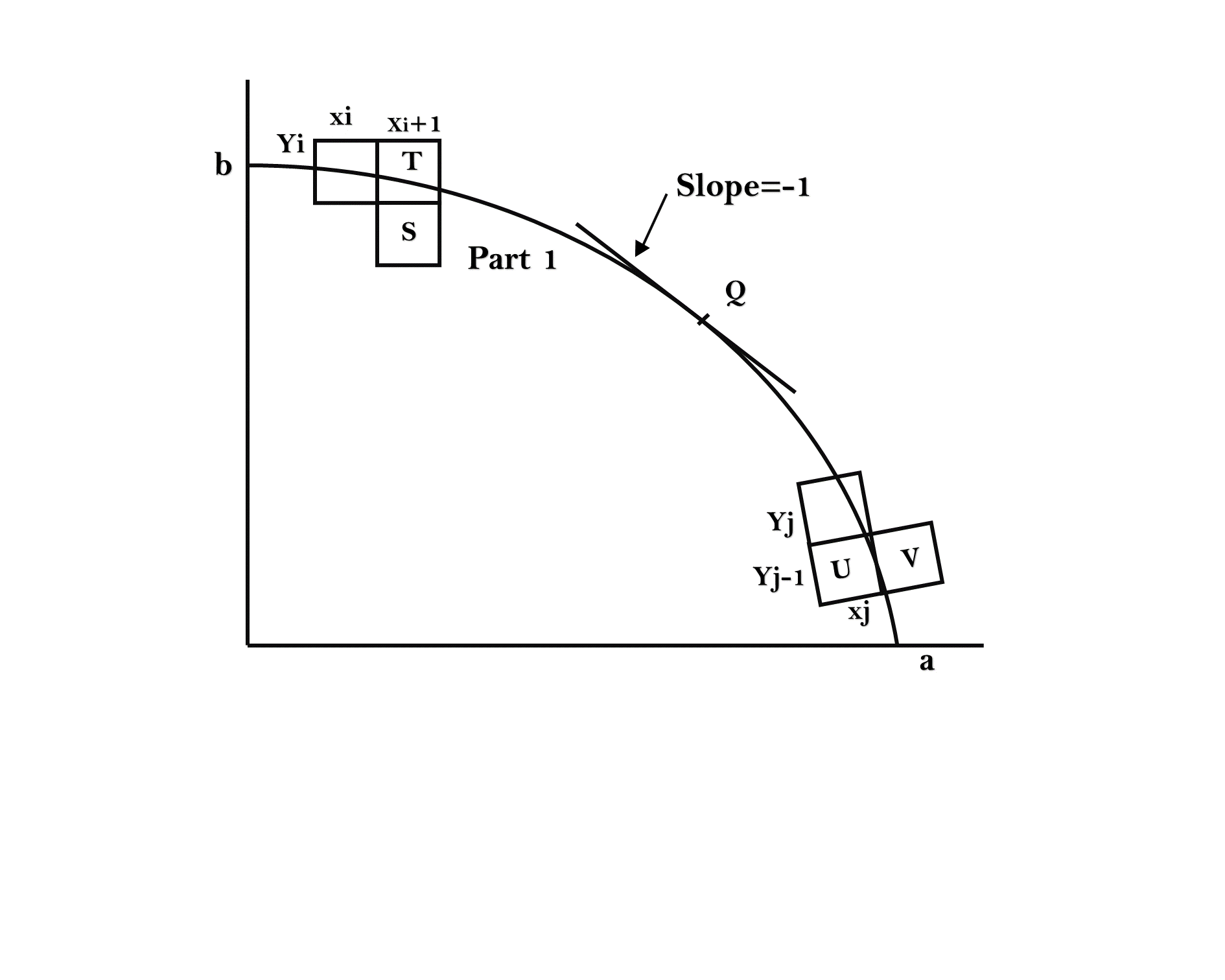

Ellipse is an elongated circle

Equation of ellipse centered at (0,0) : $x^2/a^2 + y^2/b^2 = 1$ Major Axis : $2a = 2r_x$ Minor Axis : $2b = 2r_y$

Semi-Major Axis : $a = r_x$ Semi-Minor Axis : $b = r_y$

$b^2x^2 + a^2y^2 = a^2b^2$ $b^2x^2 + a^2y^2 - a^2b^2 =0$

• dk : $d_k = (r_y)^2x^2 + (r_x)^2y^2 - (r_x)^2(r_y)^2$
  • dk=0 point lies on ellipse
  • dk<0 point lies inside ellipse
  • dk>0 point lies outside ellipse

Major Difference in Ellipse

1. In $x^2/r_x^2 + y^2/r_y^2 = 1$ -> $x=0$ : $y=r_y$ and $y=0$ : $x=r_x$
   • in ellipse $r_x \neq r_y$
   • in circle $r_x = r_y$

Difference between Circle and Ellipse

• Circle has 8-way symmetry and Ellipse has 4-way symmetry
• In circle we need to plot only 1 Octant of any quadrant, but, in ellipse we need to plot 2 octants i.e. 1 complete quadrant to plot entire ellipse.
• because in ellipse half-quadrant(octant) points (x,y) not complete the other half-quadrant(octant) by swapping (x=y , y=x). So we need to make one quadrant complete i.e. not stop when x>=y

CGMM Lecture 18 | Midpoint Ellipse Drawing Algorithm(Derivation) Part 2 - Hindi/English

Filled Area Primitive-GFG

Filled Area primitives are used to filling solid colors to an area or image or polygon. Filling the polygon means highlighting its pixel with different solid colors. Following are two filled area primitives:

1. Seed Fill Algorithm
2. Scan Fill Algorithm

Seed Fill Algorithm:

In this seed fill algorithm, we select a starting point called seed inside the boundary of the polygon. The seed algorithm can be further classified into two algorithms: Flood Fill and Boundary filled.

Polygon Filling Algorithm - Boundary Fill Algorithm Part-1 Explained in Hindi l Computer Graphics

The Boundary Fill Algorithm is used in computer graphics to fill a region with a specific color, starting from a seed point inside the region. The algorithm checks the neighboring pixels and changes their color if they are not the boundary color and not the fill color. This process continues recursively or iteratively until the entire region is filled.

Applications:

• Used in paint programs to fill closed shapes.
• Useful in image processing for region labeling.

Types:

• 4-Connected: Fills only the 4 neighboring pixels (left, right, top, bottom).

// f = color to be filled
// b = color of existing boundary
// getpixel() return the color of a pixel
// putpixel() change color of the pixel

boundary(x,y,f,b){
  if( getpixel(x,y)!=b && getpixel(x,y)!=f ){

  putpixel(x,y,f)

  // horizontally and vertically
  boundary(x+1, y, f, b) // right
  boundary(x, y+1, f, b) // up
  boundary(x-1, y, f, b) // left
  boundary(x, y-1, f, b) // down

  }
}

Polygon Filling Algorithm - Boundary Fill Algorithm Part-2 Explained in Hindi l Computer Graphics

Problem with 4-neighboring algorithm

Initial Grid wit B=black color.
      B B B B
      B     B
      B     B B B
      B B B     B
      B f   B
      B B B B
Let we start from point 'f'

      B B B B
      B     B
      B     B B B
      B B B f f B
      B f f B
      B B B B

After Filling the four pixels, it will think that, it has complete all the pixels of the polygon, but in actuall it is not able to go to the other part of the polygon, that should be traversed diagonally

• 8-Connected: Fills all 8 surrounding pixels.

// f = color to be filled
// b = color of existing boundary
// getpixel() return the color of a pixel
// putpixel() change color of the pixel

boundary(x,y,f,b){
  if( getpixel(x,y)!=b && getpixel(x,y)!=f ){

  putpixel(x,y,f)

  // horizontally and vertically
  boundary(x+1, y, f, b) // right
  boundary(x, y+1, f, b) // up
  boundary(x-1, y, f, b) // left
  boundary(x, y-1, f, b) // down

  // diagonally
  boundary(x-1, y-1, f, b) // left-down
  boundary(x-1, y+1, f, b) // left-up
  boundary(x+1, y-1, f, b) // right-down
  boundary(x+1, y+1, f, b) // right-up

  }
}

This algorithm is simple but can be inefficient for large areas, as it may require a lot of recursive calls or iterations.

Polygon Filling Algorithm - Flood Fill Algorithm Explained in Hindi l Computer Graphics Course

Problem with Boundary Fill: Boundary Fill Algorithm is limited to boundaries of a single, consistent color. If the boundary consists of different colors or patterns, the Boundary Fill algorithm may not work correctly. Additionally, the algorithm does not overwrite the boundary color, which can be a limitation when dealing with complex or multicolored boundaries.

Solution: Flood Fill Algorithm: To overcome these limitations, the Flood Fill Algorithm is used. Unlike Boundary Fill, Flood Fill doesn’t rely on a single boundary color. Instead, it uses the concept of a target color (the color you want to replace) and a replacement color (the color with which you want to fill the region).

• Target Color (Old Color): The color that needs to be changed (e.g., White).
• Replacement Color: The new color to apply to the region.

Types:

• 4-Connected Flood Fill: Only the four neighboring pixels (left, right, top, bottom) are checked.
• 8-Connected Flood Fill: All eight surrounding pixels (including diagonals) are checked.

Applications:

• Used in paint programs for filling bounded regions.
• Employed in image processing tasks such as object recognition or segmentation.
• Useful in game development, e.g., to determine the area controlled by a player.

Initial Grid filled with color W=white ('' represent as blank) color.
      B B B B
      B     G
      B     G G B
      B G G     B
      G   n B
      B B B B

Let we start from point 'n'
      B B B B
      B n n B
      B n n B B B
      B B B n n B
      B n n B
      B B B B

After Filling the four pixels, it will think that, it has complete all the pixels of the polygon, but in actuall it is not able to go to the other part of the polygon, that should be traversed diagonally

Boundary()

// n = new color
// o = old color

flood(x,y,n,o){
  if( getpixel(x,y) == o){

  putpixel(x,y,n)

  // horizontally and vertically
  flood(x+1, y, n, o) // right
  flood(x, y+1, n, o) // up
  flood(x-1, y, n, o) // left
  flood(x, y-1, n, o) // down

  // diagonally
  flood(x-1, y-1, n, o) // left-down
  flood(x-1, y+1, n, o) // left-up
  flood(x+1, y-1, n, o) // right-down
  flood(x+1, y+1, n, o) // right-up

  }
}

What is 2D Translation Explained in Hindi l Computer Graphics Course

2D Translation in Computer Graphics

2D Translation is a geometric transformation used to move an object from one location to another in a 2D plane. This operation is defined by adding a translation vector to the original coordinates of a point.

Translation Process:

• Original Point (A): Let’s say we have a point A with coordinates (x, y) in the 2D plane.
• Translation Vector (T): The translation vector is represented as (Tx, Ty), where:
  • Tx is the horizontal shift (along the x-axis).
  • Ty is the vertical shift (along the y-axis).
• Translated Point (A’): The new position of the point A after translation is A' with coordinates (x', y').

Mathematical Formula:

The translation of point A(x, y) by translation vector (Tx, Ty) is calculated as:

A' = A + T

┌    ┐   ┌    ┐   ┌    ┐
│ x' | = │ x' | + │ x' |
| y' |   | y' |   | y' |
└    ┘   └    ┘   └    ┘

Simply x’ = x + Tx y’ = y + Ty

So, the translated point A' has coordinates (x', y').

    |
  __  |..............• A'
   |  |              . (x',y')
  Ty  |              .
   |  |......• A     .
  --  |      .(3, 4) .
    |__________________
           |---Tx--|

Given: (x, y) = (3, 4) (Tx, Ty) = (5, 2)

Find (x’, y’)

x’ = 3 + 5 = 8 y’ = 4 + 2 = 6

So, the translated point A’ has coordinates (8, 6)

2D-Transformation

Transformation

$x -> x^$ $y -> y^$

OpenGL

1. Translation

Note not found

$x^ = x + t_x$ $y^ = y + t_y$

glTranslatef(tx, ty, 0.0) // (through x-axis, through y-axis,through z-axis)

2. Rotation

Note not found

about origin $x^=x.Cosθ - y.Sinθ$ $y^=x.Sinθ + y.Cosθ$

glRotatef(θ,0,0,1) // (Angle, around x-axis, around y-axis, around z-axis)

about pivot point : Translate to origin -> Rotate about Origin -> Translate to original position $x^ = ((x - x_p)Cosθ - (y - y_p)Sinθ) + x_p$ $y^ = ((x - x_p)Sinθ + (y - y_p)Cosθ) + y_p$

glTranslatef(xp, yp, 0.0)
glRotatef(θ,0,0,1)
glTranslatef(-xp, -yp, 0.0)

Derivation

Step 1 : Translate the pivot to origin

• $x_1 = x - x_p$ , $y_1 = y - y_p$ Step 2 : Rotate about origin
• $x_2 = x_1Cosθ - y_1Sinθ$ , $y_2 = x_1Sinθ + y_1Cosθ$ Step 3 : Translate the pivot point to original position
• $x_3 = x_2 + x_p$ , $y_3 = y_2 + y_p$

Substitute x2 and y2 from step 2

• $x_3 = (x_1Cosθ - y_1Sinθ) + x_p$ , $y_3 = (x_1Sinθ + y_1Cosθ) + y_p$ Substitute x and y from step 1
• $x_3 = ((x - x_p)Cosθ - (y - y_p)Sinθ) + x_p$ , $y_3 = ((x - x_p)Sinθ + (y - y_p)Cosθ) + y_p$

3. Scaling

Note not found

About the Origin $x^ = x.S_x$ $y^=y.S_y$

glScalef(Sx, Sy, 1.0) // (x-axis scaleFactor, y-axis scaleFactor,z-axis scaleFactor)

About fixed Point: Translate to origin -> Scale about Origin -> Translate to original position $x^ = (x-x_f).S_x+x_f$ $y^=(y-y_f).S_y+y_f$

glTranslatef(xp, yp, 0.0)
glScalef(Sx, Sy, 1.0)
glTranslatef(-xp, -yp, 0.0)

4. Reflections

Note not found

Original Position -> First Quadrant $(x^=x, y^=x)$

glScalef(1,1,1) // (about x-axis, about y-axis, about z-axis)

Reflection about x axis -> Second Quadrant $(x^=x, y^=-y)$

glScalef(1,-1,1)

Reflection about y axis -> Third Quadrant $(x^=-x, y^=y)$

glScalef(-1,1,1)

Reflection about Origin -> Fourth Quadrant $(x^=-x, y^=-y)$

glScalef(-1,-1,1)

5. Shears

Note not found

about x-axis : Shear in x-direction Proportional to y-direction $x^ = x +h_x.y$ $y^=y$

about y-axis : Shear in y-direction Proportional to x-direction $x^ = x$ $y^=y + h_y.x$

2-D Matrix Representation

1. Translation

$$ \begin{bmatrix} x’ \ y’ \ \end{bmatrix}

\begin{bmatrix} x \ y \ \end{bmatrix} + \begin{bmatrix} t_x \ t_y \ \end{bmatrix} $$

2. Rotation (about origin):

$$ \begin{bmatrix} x’ \ y’ \end{bmatrix}

\begin{bmatrix} \cos \theta & -\sin \theta \ \sin \theta & \cos \theta \end{bmatrix} \begin{bmatrix} x \ y \end{bmatrix} $$

3. Scaling (about origin):

$$ \begin{bmatrix} x’ \ y’ \end{bmatrix}

\begin{bmatrix} S_x & 0 \ 0 & S_y \end{bmatrix} \begin{bmatrix} x \ y \end{bmatrix} $$

4. Reflection:

• About x-axis: $$ \begin{bmatrix} x’ \ y’ \end{bmatrix}

  \begin{bmatrix} 1 & 0 \ 0 & -1 \end{bmatrix} \begin{bmatrix} x \ y \end{bmatrix}

• About y-axis:

$$ \begin{bmatrix} x’ \ y’ \end{bmatrix}

\begin{bmatrix} -1 & 0 \ 0 & 1 \end{bmatrix} \begin{bmatrix} x \ y \end{bmatrix} $$

• About origin:

$$$ \begin{bmatrix} x’ \ y’ \end{bmatrix} = \begin{bmatrix} -1 & 0 \ 0 & -1 \end{bmatrix} \begin{bmatrix} x \ y \end{bmatrix} $$

5. Shear:

• Along x-axis (shear factor = ( h )):

  $$ \begin{bmatrix} x’ \ y’ \end{bmatrix}

  \begin{bmatrix} 1 & h \ 0 & 1 \end{bmatrix} \begin{bmatrix} x \ y \end{bmatrix} $$

• Along y-axis (shear factor = ( h )): $$$

 \begin{bmatrix}
 x' \\
 y'
 \end{bmatrix}
 =
 \begin{bmatrix}
 1 & 0 \\
 h & 1
 \end{bmatrix}
 \begin{bmatrix}
 x \\
 y
 \end{bmatrix}
 $$

Homogeneous Coordinates

In computer graphics, homogeneous coordinates are used to represent points and transformations in a way that allows for more efficient matrix-based operations. By adding an extra dimension (w-coordinate), transformations like translation, rotation, scaling, and perspective projection can be represented uniformly as matrix multiplications. This extra coordinate enables the system to handle a variety of transformations in a compact, consistent manner.

In 2D space:

• A point $(x, y)$ in Cartesian coordinates can be represented in homogeneous coordinates as $(x, y, 1)$.
• The transformation matrix can then operate in 3D space, simplifying composition of transformations.

The general form of a point in 2D homogeneous coordinates is:

$$ \begin{bmatrix} x \ y \ w \end{bmatrix} $$

where (w) is typically set to 1 for regular 2D points. To convert a homogeneous point back to Cartesian coordinates, you divide by (w):

$$ (x, y) = \left( \frac{x}{w}, \frac{y}{w} \right). $$

Common 2D Transformations in Homogeneous Coordinates

1. Translation

In Cartesian coordinates, translation requires adding $t_x$ and $t_y$ to $x$ and $y$, respectively. In homogeneous coordinates, this can be done with matrix multiplication:

$$ \begin{bmatrix} x’ \ y’ \ 1 \end{bmatrix} = \begin{bmatrix} 1 & 0 & t_x \ 0 & 1 & t_y \ 0 & 0 & 1 \end{bmatrix} \begin{bmatrix} x \ y \ 1 \end{bmatrix} $$

2. Rotation (about the origin)

To rotate a point around the origin by an angle (\theta), we use the following matrix:

$$ \begin{bmatrix} x’ \ y’ \ 1 \end{bmatrix} = \begin{bmatrix} \cos \theta & -\sin \theta & 0 \ \sin \theta & \cos \theta & 0 \ 0 & 0 & 1 \end{bmatrix} \begin{bmatrix} x \ y \ 1 \end{bmatrix} $$

3. Scaling (about the origin)

Scaling by factors (S_x) and (S_y) along the x- and y-axes, respectively, is represented by:

$$ \begin{bmatrix} x’ \ y’ \ 1 \end{bmatrix} = \begin{bmatrix} S_x & 0 & 0 \ 0 & S_y & 0 \ 0 & 0 & 1 \end{bmatrix} \begin{bmatrix} x \ y \ 1 \end{bmatrix} $$

4. Reflection

Reflection transformations can also be achieved in homogeneous coordinates. For example:

• Reflection about the x-axis:

  $$ \begin{bmatrix} x’ \ y’ \ 1 \end{bmatrix} = \begin{bmatrix} 1 & 0 & 0 \ 0 & -1 & 0 \ 0 & 0 & 1 \end{bmatrix} \begin{bmatrix} x \ y \ 1 \end{bmatrix} $$

• Reflection about the y-axis:

  $$ \begin{bmatrix} x’ \ y’ \ 1 \end{bmatrix} = \begin{bmatrix} -1 & 0 & 0 \ 0 & 1 & 0 \ 0 & 0 & 1 \end{bmatrix} \begin{bmatrix} x \ y \ 1 \end{bmatrix} $$

• Reflection about the origin:

  $$ \begin{bmatrix} x’ \ y’ \ 1 \end{bmatrix} = \begin{bmatrix} -1 & 0 & 0 \ 0 & -1 & 0 \ 0 & 0 & 1 \end{bmatrix} \begin{bmatrix} x \ y \ 1 \end{bmatrix} $$

5. Shear

• Shear along x-axis with factor ( h ):

  $$ \begin{bmatrix} x’ \ y’ \ 1 \end{bmatrix} = \begin{bmatrix} 1 & h & 0 \ 0 & 1 & 0 \ 0 & 0 & 1 \end{bmatrix} \begin{bmatrix} x \ y \ 1 \end{bmatrix} $$

• Shear along y-axis with factor ( h ):

  $$ \begin{bmatrix} x’ \ y’ \ 1 \end{bmatrix} = \begin{bmatrix} 1 & 0 & 0 \ h & 1 & 0 \ 0 & 0 & 1 \end{bmatrix} \begin{bmatrix} x \ y \ 1 \end{bmatrix} $$

These transformations allow us to manipulate 2D points using matrix multiplications, making it easier to combine multiple transformations into a single composite transformation matrix.

5.8- Scan Line Polygon Area Filling Algorithm In Computer Graphics

Polygon Area Filling Algorithm:

1. Seed filling algorithm
2. Scan line algorithm

Disadvantage of Seed fill algorithm ( So wee need Scan line algorithm )

1. they use 4-connected and 8-connected algorithm. In 4-connected algorithm, it is not able to fille complete area always. In 8-connected, if the area is too large, it also not work.
2. There we make stack and sometime the stack got too large Note:- for small area, boundary fill and flood fill are good but not for big area

Scan Line

Steps

1. Locate the intersection points of the Scan Line with the polygon Edges
2. Pairing Intersection Points
3. Move down Side As per Scan Line and Sort all Pairs
4. All Pairs are sorted From Ymax to Ymin (Top to down)

{(x0,y0),(x1,y1)} , {(x2,y2),(x3,y3)} , {(x4,y4),(x5,y5)} .....

Edge List
┌────┐
├────┤
├────┤
├────┤
└────┘

5. Sides Get sorted on Intersection point bases
6. Area filling starts Now

Important: If the scan line intersect at the vertex of Polygon, then if the two lines making vertex line on same side, will count as two different points i.e the coordinate will count two times.

Coherence Property : -> Relating Property of One Scene to Another Part of Scene Slope of Line is m m = (y2-y1)/(x2-x1) = Δy/Δx,
Here Δy=-1 (Always , because scan line by line from top do bottom) Δx= -1/m

yk+1 = yk - 1 xk+1 = xk - 1/m

Vector and Character generation - lecture 9/ computer graphics

[Two Dimensional Transformation]

Transformation - Transform every point on an object according to certain rule.

The point Q is the image of P under the transformation T,

x -> x`
y -> y'

Anti Aliasing | Computer Graphics Lectures in Hindi

Super sampling

Vector and Character generation - lecture 9/ computer graphics

There are 3 methods for generating characters with software impemntations

1. Stroke method
2. Vector method / bitmap method
3. Star bust method

1. Stroke Method In this method, we use a sequence of line drawing functions and arc functions to generate characters.

• we can generate a sequence of character by assigning starting and ending point of line or arc.
• By using this method various forms of character can be generated by changing the values/parameters in the line and arc functions
• Disadvantages- It produce aliased character

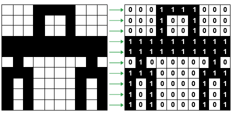
2. Vector or Bitmap Method

It is also known as dot matrix because in this method characters are represented by an array of dots in the matrix form.

• It’s a 2D array having columns and rows.
• Font size of Character can be increased by increasing the size of array.
• Higher Resolution devices may use character array 100x100
• Each dot in the matrix is a pixel
• The character is placed on the screen by copying pixel values from the character array and value of the pixel controls the intensity of the pixel

Star bust Method

• A fixed pattern of line is used to generated the characters
• In this method we use a combination of 24bit line segment
• In 24 bit line segment code each bit represent a single line
• To highlight a line we put corresponding bit 1 in 24 bit line segment code and 0 other wise

Character `A`

 24 23 22 21 20 19 18 17 16 15 14 13 12 11 10 9 8 7 6 5 4 3 2 1
[ 0  0  1  1  0  0  0  0  0  0  1  0  1  1  0 0 1 1 1 0 0 0 0 1]

• Disadvantages

1. 24 bits are required to represent a character hence more memory is required
2. Poor character quality due to limited face
3. Worst for curve shaped character
4. Requires code conversion software to display character from its 24 bits code.

line attributes in computer graphics | computer graphics notes

Line has 3 basic attributes:

1. Line Width
2. Line Color
3. Line type

Line Width:

• The line width depends on capability of the device to display it
• In raster scan display the standard width line (or default line) is drawn with one pixel at each sample position.
• To draw thicker line another parallel line is drawn adjacent to the first one.

Line Color

• When we draw a line the default color of the line is displayed like for example the color of line drawn in Microsoft paint is black. • The number of color choices depends on the number of bits available per pixel in the frame buffer. • In Microsoft Paint we are given a drop down area to choose from-different color options.

Line Types

• There are 3 types of lines:

1. Solid line
2. Dashed line
3. Dotted Line

Solid Line:

• Solid line is the default line which is drawn with complete solid section for the length specified.

Dashed Line:

• To draw dashed line we generate an inter-dash spacing that is equal to the length of the solid sections.
• So basically we specify the full length of the line and then length of the dashed solid section and the length of the spacing which is usually in the color of background.

Dotted Line:

• To draw a dotted line very short dashes are drawn
• In this dotted line the spacing between the dots(small dashes) can be equal to or greater than the dash size.

Commands for Line attribute

- The command to set line widht is:
SetLinewidthScaleFactor(lw)

- The command to choose the color is (in PHIGS)
SetPolylineColorlndex (lc)

- The Command To set line type attribute (in PHIGS)

Note: PHIGS - Programmer’s Hierarchical Interactive Graphics System

# Homogeneous Coordinate Explained in Hindi l Computer Graphics